Thread // ARCHITECTURE / EFFICIENCY

Token Deep Memory.

From gist embeddings to token averaging — compressing the input sequence before the transformer sees it. A k=4 model reaches the same loss as baseline at 42% fewer FLOPs, and linear probes reveal why: averaging trades syntax for semantics.

6 POSTS

The Quadratic Wall

Standard self-attention scales quadratically in context length because every token attends to every other token. At 128K128\text{K} tokens, the attention matrix holds 1616 billion entries. At 1M1\text{M} tokens — a plausible requirement for long-horizon agents — it holds 11 trillion. The memory and compute cost is prohibitive even on modern hardware.

Linear attention and sparse attention are partial solutions. Linear attention approximates the softmax kernel, trading exact computation for efficiency but degrading on tasks that require precise token retrieval. Sparse attention restricts the attention pattern to local windows or learned patterns, but must decide ahead of time which tokens are worth attending to — a decision that can only be made correctly with the full context in view.

Memory as the real problem

The core issue is not attention computation — it is the assumption that all past tokens deserve equal representation fidelity. Human working memory does not store every sensory event at full resolution; it stores compressed summaries and retains high-fidelity traces only for events that were subsequently reinforced or retrieved.

A model that mimics this would maintain most historical context in a compressed state, with the option to reconstruct high-fidelity fragments on demand. The quadratic blowup disappears because the dense attention matrix is replaced by a much smaller matrix over compressed summaries.
Gist Embeddings and Retrieval

In our architecture, every kk consecutive historical tokens are compressed into a single gist vector by a learned pooling operation. The gist preserves mean semantic content while discarding positional and high-frequency token-level variation. The compression schedule is adaptive: regions of high gradient signal during training are compressed more slowly; redundant stretches collapse aggressively.

Formally, for a block of token hidden states h1,,hkh_1, \ldots, h_k, the gist is computed as:

hˉ=Pool(h1,,hk)=Wmean(h1,,hk)+b\bar{h} = \text{Pool}(h_1, \ldots, h_k) = W \cdot \text{mean}(h_1, \ldots, h_k) + b

where WW and bb are learned. The pooling can be replaced with a small attention mechanism over the block for higher fidelity at modest cost.

Retrieval on demand

Attention over gists runs in O(n/k)O(n/k) time — linear in the number of compressed blocks rather than the number of raw tokens. When the model's attention pattern signals that a compressed region is load-bearing for the current prediction, a retrieval head reconstructs an approximation of the original token sequence from the gist embedding.

This two-tier system — compressed storage, on-demand decompression — mirrors episodic memory architectures observed in biological neural systems, where the hippocampus stores compressed event representations and reconstructs detail when a retrieval cue matches the stored pattern.

Open questions

The current design treats compression granularity kk as a fixed hyperparameter. An obvious extension is a learned, dynamic kk that varies based on local information density. We are also investigating whether gist vectors can serve as addressable keys in an external memory bank, enabling context windows that extend across multiple inference sessions.

Token Averaging — Compressing the Input Sequence

The gist embedding idea from the previous post assumed a learned compression. We step back and ask a simpler question first: what if we compress the input sequence before the transformer even sees it — by plain averaging of neighbouring token embeddings?

Token averaging is static and parameter-free. Before the first transformer layer, every kk consecutive token embeddings are collapsed into a single mean vector. The transformer then runs on a sequence that is k×k\times shorter.

Raw tokens:   [t1, t2, t3, t4, t5, t6, t7, t8]

k=2 average:  [avg(t1,t2), avg(t3,t4), avg(t5,t6), avg(t7,t8)]   → 4 positions
k=4 average:  [avg(t1..t4),            avg(t5..t8)]               → 2 positions

For a raw sequence of length LL and window kk, the transformer processes L/kL/k positions. The training objective remains next-token prediction: a compressed position predicts the first token of the next window. This keeps validation loss directly comparable to a standard model.

Two knobs, two different stories

It matters whether you spend the compression on shortening the transformer or widening the effective context:

  • Reduce cost — keep the raw context fixed, shrink the transformer to L/kL/k positions. Each step is cheaper, so a fixed compute budget buys more steps.
  • Extend context — feed a k×k\times longer raw sequence so the transformer still processes LL positions but covers k×Lk \times L raw tokens. Same cost per step, wider window.

A core finding is that these two uses behave very differently. The next post has the numbers.

The 42% Result

We run the controlled experiment at 50M parameters on an OLM transformer with RoPE, SwiGLU FFN, and tied embeddings, trained on FineWeb.

Iso-FLOPs design

Three configurations isolate the two uses of compression:

Model Sequence length kk Transformer LL Cost/seq Interpretation
k=1k = 1 (baseline) 10241024 11 10241024 1×1\times reference
k=2k = 2 20482048 22 10241024 1×1\times extend context (same transformer, 2×2\times raw window)
k=4k = 4 10241024 44 256256 14×\sim \tfrac{1}{4}\times reduce cost (4×4\times shorter transformer)

The k=2k = 2 model sees 2×2\times more raw tokens but has the same transformer length as baseline. The k=4k = 4 model has a 4×4\times shorter transformer and uses the savings to see 5×\sim 5\times more raw tokens within the same FLOPs budget.

The headline number

At iso-FLOPs (1.95×10171.95 \times 10^{17}), the three models reach:

Model Tokens at iso-FLOPs Eval loss
k=1k = 1 1.00B1.00\text{B} 5.39985.3998
k=2k = 2 2.01B2.01\text{B} 5.43415.4341
k=4k = 4 4.96B4.96\text{B} 5.18305.1830

The k=4k = 4 model reaches k=1k = 1's final loss at 42%\sim 42\% fewer FLOPs (1.13×10171.13 \times 10^{17} vs 1.95×10171.95 \times 10^{17}). The k=2k = 2 model, despite seeing 2×2\times more raw tokens, shows no improvement — it actually trails the baseline slightly.

Loss vs FLOPs — the central figure

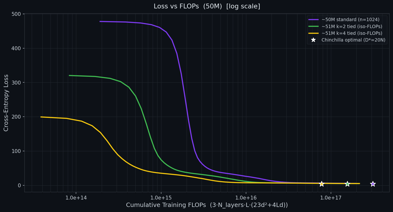
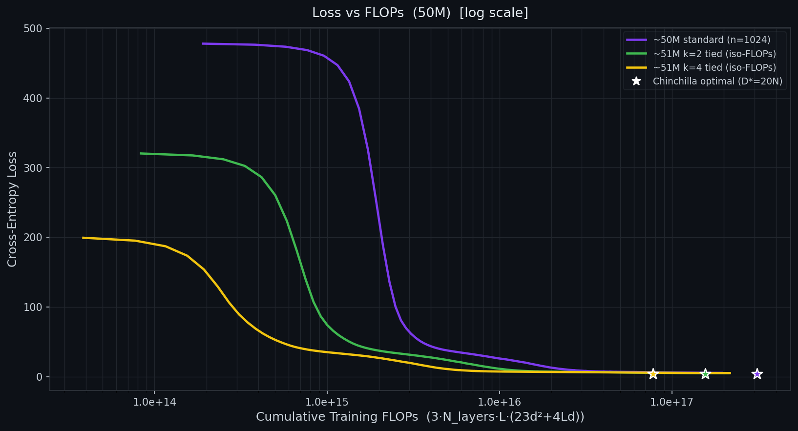
At equal FLOPs, k=4k = 4 (yellow) sits well below both k=1k = 1 (purple) and k=2k = 2 (green).

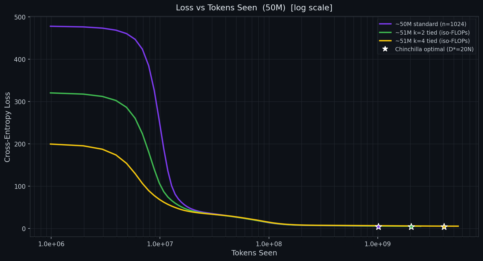
Loss vs tokens seen

k=4k = 4 consumes 5.5×\sim 5.5\times more raw tokens than k=1k = 1 for the same compute (each pass is 4×\sim 4\times cheaper).

The punchline

The contrast between k=2k = 2 and k=4k = 4 is the key insight: the benefit comes from reducing the number of transformer positions, not from exposing the model to more raw data. When compute per sequence is held constant (the k=2k = 2 case), the information lost to averaging roughly cancels the advantage of seeing more tokens. When the transformer is shortened (the k=4k = 4 case), the compute savings dominate.

Loss vs FLOPs on log scale

k=4k = 4's advantage is present throughout training, not just at the endpoint.

This is a compute-efficiency story, not a data-efficiency story.

Capacity threshold

At 8M8\text{M} parameters, averaging hurts — the small model spends its limited capacity just coping with the blended representations rather than learning from them. Decoding averaged ("superposed") embeddings is itself a skill that costs model capacity. The technique needs a minimum scale to pay off.

What Averaging Destroys

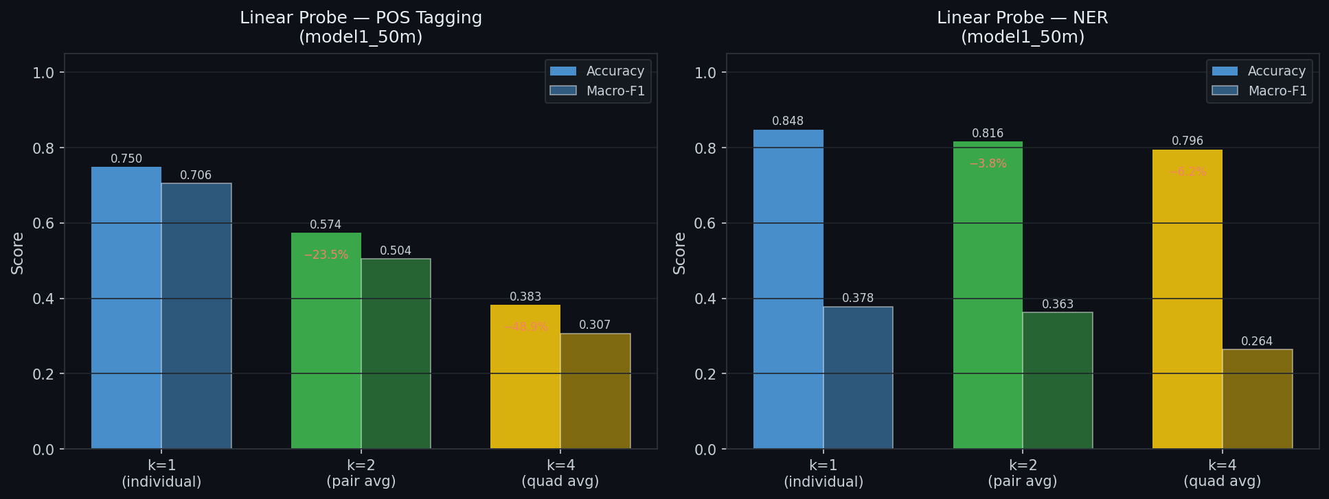
To understand why averaging behaves this way, we trained linear probes on top of averaged embeddings and measured how well linguistic structure survives compression. Two tasks from CoNLL-2003: POS tagging (syntactic structure) and NER (lexical/semantic structure).

Syntax degrades fast, semantics is robust

Task k=1k = 1 k=2k = 2 k=4k = 4 Random control
POS tagging (accuracy) 0.7500.750 0.5740.574 0.3830.383 0.7350.735
NER (accuracy) 0.8480.848 0.8160.816 0.7960.796 0.8050.805

POS accuracy falls from 0.7500.750 to 0.3830.383 as kk grows, dropping below the random-embedding control by k=4k = 4. Word-order- and position-sensitive structure is largely washed out by averaging — unsurprising, since pooling neighbours discards exactly the local ordering that POS depends on.

NER barely moves (0.8480.7960.848 \to 0.796) and stays above the random control even at k=4k = 4. Entity identity is carried by which words are present more than by their precise order, so it survives pooling.

Linear probe results — POS tagging vs NER across k values

POS accuracy (left) collapses with averaging while NER accuracy (right) is robust. The pattern is consistent across both accuracy and macro-F1.

The mechanistic match

This maps cleanly onto the compute results:

  • Averaged representations keep enough "what is being talked about" (semantic signal) to support language modelling cheaply
  • They sacrifice "exact local arrangement" (syntactic signal) — which is part of why aggressive kk eventually hurts

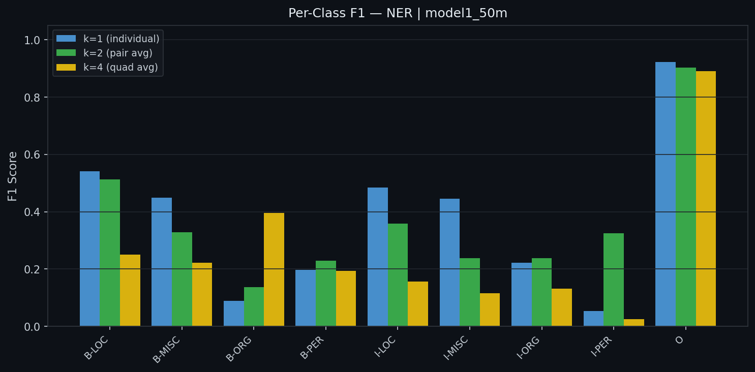
The per-class breakdowns confirm the degradation is concentrated in categories that most depend on local context, while entity-level categories are preserved.

Per-class NER F1 across k values

Per-class NER F1. The dominant "O" (non-entity) class is nearly unaffected, while entity categories degrade modestly and uniformly — no single entity type is disproportionately harmed.

This tells us where the ceiling is: token averaging works until the task demands fine-grained syntactic structure that averaging has erased.

Open Questions and Next Steps

Rigour note: the causal-masking bug

Early in the project, a bug was discovered: causal masking was not applied even though causal=True was set. Models trained under this bug performed bidirectional attention, producing artificially low loss values. Every run from before the fix is invalidated for absolute comparison. We report the corrected runs as primary results and clearly mark pre-fix experiments as exploratory.

Silent correctness bugs in the training stack can masquerade as "great results." Treating suspiciously good numbers as a red flag, not a win, saved this project from a wrong conclusion.

Limitations

  • Single primary scale (50M50\text{M}). The 42%42\% figure is demonstrated at one model size and must be re-validated as capacity grows.
  • Loss, not downstream tasks. We measure validation cross-entropy. Lower loss is necessary but not sufficient — downstream benchmarks are needed.
  • Static, uniform pooling for the main result. The headline numbers use plain mean-pooling; smarter schemes are unexplored under corrected attention.
  • Probes use input embeddings, not deep contextual states. The interpretability story is about what averaging does to the inputs the transformer receives.

What we want to try next

  1. Scale up (150M150\text{M} to 1B+1\text{B}+). Test whether the 42%\sim 42\% saving holds, grows, or erodes with capacity. Config scaffolding for 125M125\text{M}/150M150\text{M} models already exists.

  2. Find the optimal kk per scale. Larger models may tolerate more aggressive compression — or may need less. Exploratory runs at k=8,16,32,64k = 8, 16, 32, 64 show diminishing returns beyond a point.

  3. Dynamic kk scheduling. Start cheap (high kk, lots of data) and anneal to fine-grained (low kk) — combining the data reach of high kk with the representation quality of low kk.

  4. Smarter pooling schemes. The codebase supports weighted (uniform / linear / exponential / gaussian / triangular), overlapping (configurable window/stride), dynamic variable-length, and learnable averagers. These are the levers for "smarter than mean-pooling" follow-ups.

  5. Downstream evaluation. Confirm the loss improvement transfers to tasks (MMLU, HellaSwag, etc.).

  6. Compose with the rest of the stack. Averaging is orthogonal to Flash Attention, gradient checkpointing, mixed precision, and parallelism — quantify the combined effect.

The core takeaway stands: compression pays off through transformer length, not through data volume. The question now is how far this principle scales and whether smarter compression can push the efficiency frontier further.