Thread // EFFICIENCY / PRUNING

Learned Efficiency Pruning.

A weight-conditioned hypernetwork that reads out a network's redundancy directly from its weights — no data, no gradients — pruning 60–85% of neurons while strictly dominating classical heuristics.

5 POSTS

The Weight Readout Hypothesis

Most pruning methods ask the same question: which neurons matter for the data? They push examples through the network, collect activation magnitudes or gradient-based importance scores, and rank neurons by a scalar summary. The recipe — train dense, score by magnitude, remove the smallest, fine-tune — goes back to Han et al. (2015) and remains the strongest simple baseline.

Two properties unify nearly all of this work. First, the importance signal is data-dependent: you need forward passes to score a neuron. Second, the scoring is local and independent: each neuron gets a scalar rank, and interactions between neurons (and between layers) are handled only implicitly through iterative retraining.

The question we actually want to ask

We take a different stance. Instead of asking "which neurons have small activations on this data?", we ask: what does the weight matrix itself tell us about how compressible this network is?

The hypothesis is simple — a trained network's redundancy is already written into its weights. If that's true, then a small model should be able to read it out directly, without ever seeing the training data. No forward passes, no gradients, no iterative prune-retrain cycles. Just weights in, mask out.

Why this reframing matters

If redundancy is a readable property of the weights, then pruning becomes a measurement rather than an optimization. The mask is not a design choice — it is a fact about the network, discovered rather than imposed. This changes what pruning can tell us: it stops being just a compression tool and becomes an instrument for probing how much of a network's capacity is actually being used.

This is the starting point for Learned Efficiency Pruning. The next post describes the model that performs this readout.

A Weight-Conditioned Hypernetwork

Learned Efficiency Pruning (LEP) is a hypernetwork that consumes a frozen network's weight matrices and emits a keep/prune gate per neuron. The base network is never updated — only the hypernetwork's parameters are trained.

Setup

Given a trained classifier fθf_\theta with frozen weights θ\theta, we treat each prunable layer \ell with weight matrix WRn×dW_\ell \in \mathbb{R}^{n_\ell \times d_\ell} row-by-row. Row ii — the fan-in weight vector of neuron ii — becomes one token. A hypernetwork hϕh_\phi reads these tokens and emits a logit sis_i per neuron; a gate gi=σ(si)[0,1]g_i = \sigma(s_i) \in [0, 1] multiplies that neuron's output, smoothly interpolating between keeping and pruning it.

The encoder: a bidirectional LSTM

The encoder is a BiLSTM that scans the rows of each layer. This means the score for neuron ii is informed by the entire population of weight vectors in its layer — not just W,iW_{\ell, i} in isolation. A small per-layer context head summarizes each layer and is passed across layers, giving the model a cross-layer view so it can allocate sparsity between layers, not just within one.

Training stability

Stable training required a specific recipe, arrived at empirically:

  • Tanh-bounded cross-layer context — the layer-allocation signal is squashed to (1,1)(-1, 1) so no single layer can run away and starve another
  • LayerNorm + gradient clipping on the encoder
  • Final gate-layer bias initialized to +2.0+2.0 — every gate starts open, so pruning is a deliberate act of closing gates rather than the reverse
  • Zero-initialized context head — the cross-layer signal starts neutral

The objective

We minimize the task loss under a soft sparsity penalty:

L(ϕ)=E ⁣[CE ⁣(fθgϕ(x),  y)]+λ1L=1Lgˉ\mathcal{L}(\phi) = \mathbb{E}\!\left[\,\text{CE}\!\left(f_\theta \odot g_\phi(x),\; y\right)\right] + \lambda \cdot \frac{1}{L} \sum_{\ell=1}^{L} \bar{g}_\ell

where gˉ\bar{g}_\ell is the mean gate in layer \ell and gates are binarized in the forward pass with a straight-through estimator (STE). The single knob λ\lambda trades accuracy against sparsity. Because the +2.0+2.0 bias holds scores near the STE's active band, gradient reaches every neuron at once — the penalty is a smooth, global Lagrangian rather than a hard budget.

At inference, the hypernetwork needs no data and no gradients: it reads θ\theta and emits a mask.

Core Results

All MNIST experiments use a 7841024102410784 \to 1024 \to 1024 \to 10 MLP (baseline test accuracy 98.06%98.06\%) unless stated; CIFAR experiments use a convolutional backbone with an MLP head.

Weights alone encode redundancy — and the readout is deterministic

A pruner that sees only weights prunes 60–79% of the MNIST MLP at <0.1< 0.13.73.7 pp accuracy loss. Re-running the pruner from different random seeds on the same checkpoint produces essentially the same mask (alive/dead ratio σ=0.007\sigma = 0.007). Redundancy is not an artifact of a particular training run of the pruner — it is a fixed, readable property of the trained weights.

LEP strictly dominates classical heuristics

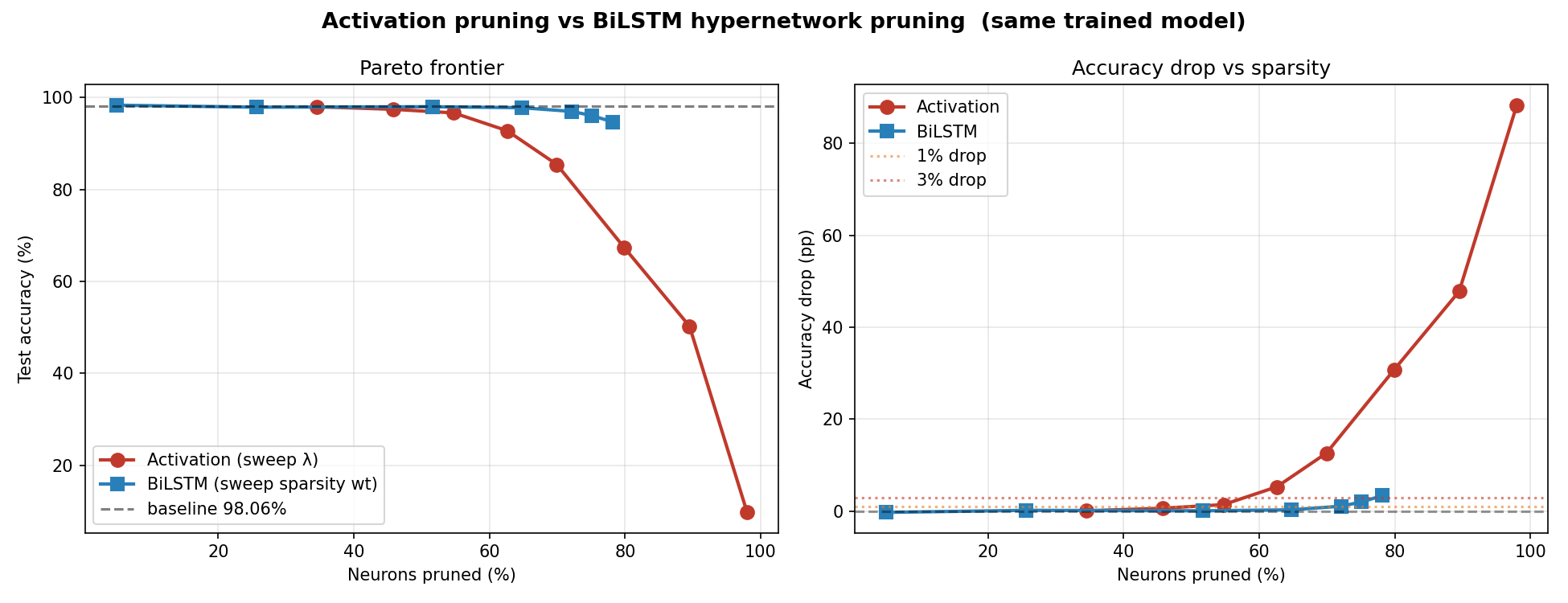
At every accuracy budget, the weight-conditioned readout prunes more than activation- or magnitude-based scoring. At a 1\leq 1 pp accuracy-drop budget, LEP removes 72%\sim72\% of neurons versus 46%\sim46\% for activation pruning. Activation pruning collapses sharply past 55%\sim55\% pruned, while LEP holds 98.0%98.0\% accuracy at 52%52\% pruned and drops only 22 pp at 75%75\%.

LEP vs activation and magnitude pruning on the same trained MNIST model

Accuracy vs fraction pruned for the same trained MNIST model. The gap is the value of scoring full weight vectors jointly rather than scalar activation summaries independently.

Bigger networks are more prunable

Sweeping hidden width on a fixed task, prunability rises monotonically with size: a width-3232 net yields 8%\sim8\% prunable, width-10241024 yields 25%\sim25\%, width-20482048 yields 51%\sim51\% (at matched penalty). This is exactly the over-parameterization story behind the lottery ticket hypothesis, here read out directly by the pruner.
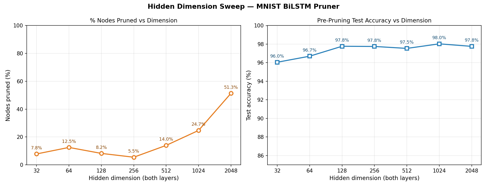
Prunability rises monotonically with hidden dimension

Fraction pruned vs hidden dimension. Redundancy — and thus prunability — scales with over-parameterization.

Width is cheap, depth is load-bearing — and weights are conserved

Holding the neuron budget fixed at 20482048 and varying shape reveals that prunability is governed by width, not depth or parameter count: a single wide layer [2048][2048] prunes to 85%\sim85\%, the medium [1024,1024][1024, 1024] to 76%\sim76\%, and a deep [512×4][512 \times 4] only to 60%\sim60\%. Yet when measured in weights rather than neurons, all three architectures converge to 240K\sim240\text{K} surviving weights — an architecture-invariant compute floor for MNIST at this accuracy.
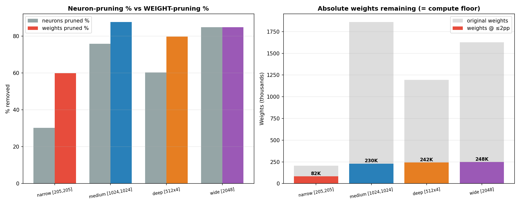
Width/depth prunability and weight conservation across architectures

Despite very different neuron-survivor counts across shapes (314314 / 490490 / 814814 for 11 / 22 / 44 layers), the surviving weight count lands near 240K\sim240\text{K} for all three 20482048-neuron nets. Width is cheap parallel redundancy; depth is sequential, load-bearing capacity. The conserved quantity is weights, not neurons.

Notably, pruning a large net down to this 240K\sim240\text{K} floor does not reach the true minimum: a network trained small from scratch reaches comparable accuracy with 3×\sim3\times fewer weights. Pruning recovers a redundant solution, not the minimal one — consistent with Liu et al. (2019).

The method transfers; the mask does not

A pruner trained on network AA, applied frozen to network BB, is catastrophic (28\sim28 pp drop). Retraining the same architecture of pruner on BB recovers within 4\sim4 pp. Redundancy is real and findable in every network, but its location is idiosyncratic to each network's weights — each lives in its own permutation frame. LEP is a reliable procedure, not a portable answer.
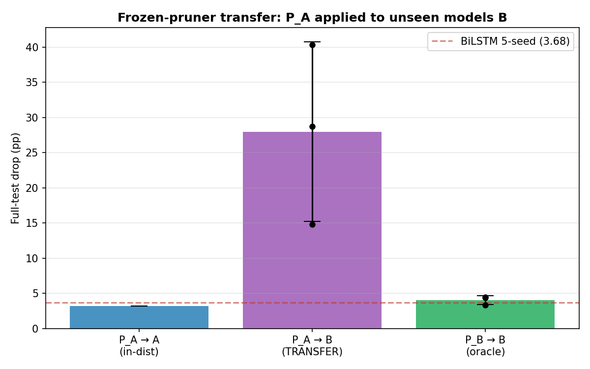
Frozen-pruner transfer experiment

A frozen pruner transferred across networks performs far worse than an oracle pruner retrained on the target — the redundancy structure does not generalize, even though the method does.
Why RL Fails — and Why Soft Beats Hard

The reinforcement-learning framing is structurally degenerate

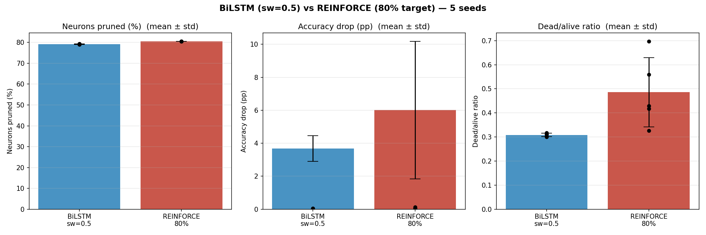
Sequential pruning — "decide neuron by neuron" — invites a reinforcement-learning treatment, and we tested it thoroughly: REINFORCE, PPO, actor-critic, Bernoulli policies, entropy and chunk-size variants. Every variant matched or lost to the differentiable hypernetwork.

BiLSTM vs REINFORCE comparison at 80% pruning target

Best-case RL (actor-critic) sits at 4.71±1.554.71 \pm 1.55 pp drop versus LEP's 3.68±0.793.68 \pm 0.79 pp at 80%\sim80\% pruned, with far higher variance.

This is not a tuning failure — it is structural. On a frozen model, the per-step reward telescopes, so the episode return depends only on the final set of kept neurons, not the order they were chosen. The pruning MDP therefore has a path-independent return: it is static subset selection wearing a sequential costume.

A problem with path-independent return has no credit-assignment structure for RL to exploit, so a direct differentiable optimizer provably dominates. The one regime where this doesn't hold is pruning during training, when the weights co-adapt to each masking decision and the return stops telescoping — which is exactly where we point future work.

Soft global penalty beats hard budget

A natural "knob-free" alternative to λ\lambda is a hard top-KK budget with an STE. We implemented it carefully and found it brittle and structurally weaker: even fully debugged, it reaches only 35%\sim35\% pruned at iso-accuracy versus LEP's 76%\sim76\% — roughly 2.6×2.6\times worse.

The reason is general: a hard budget with a centered STE gives gradient only to the few neurons sitting near the moving threshold (boundary-local), whereas the soft λ\lambda penalty keeps every neuron's gate in the active band and optimizes the whole subset jointly (global gradient). Removing a hyperparameter by switching to a hard constraint trades a sweep for both a stability-guardrail stack and a worse optimizer. Sweep-free is not the same as better.

λ\lambda is well-behaved and predictable

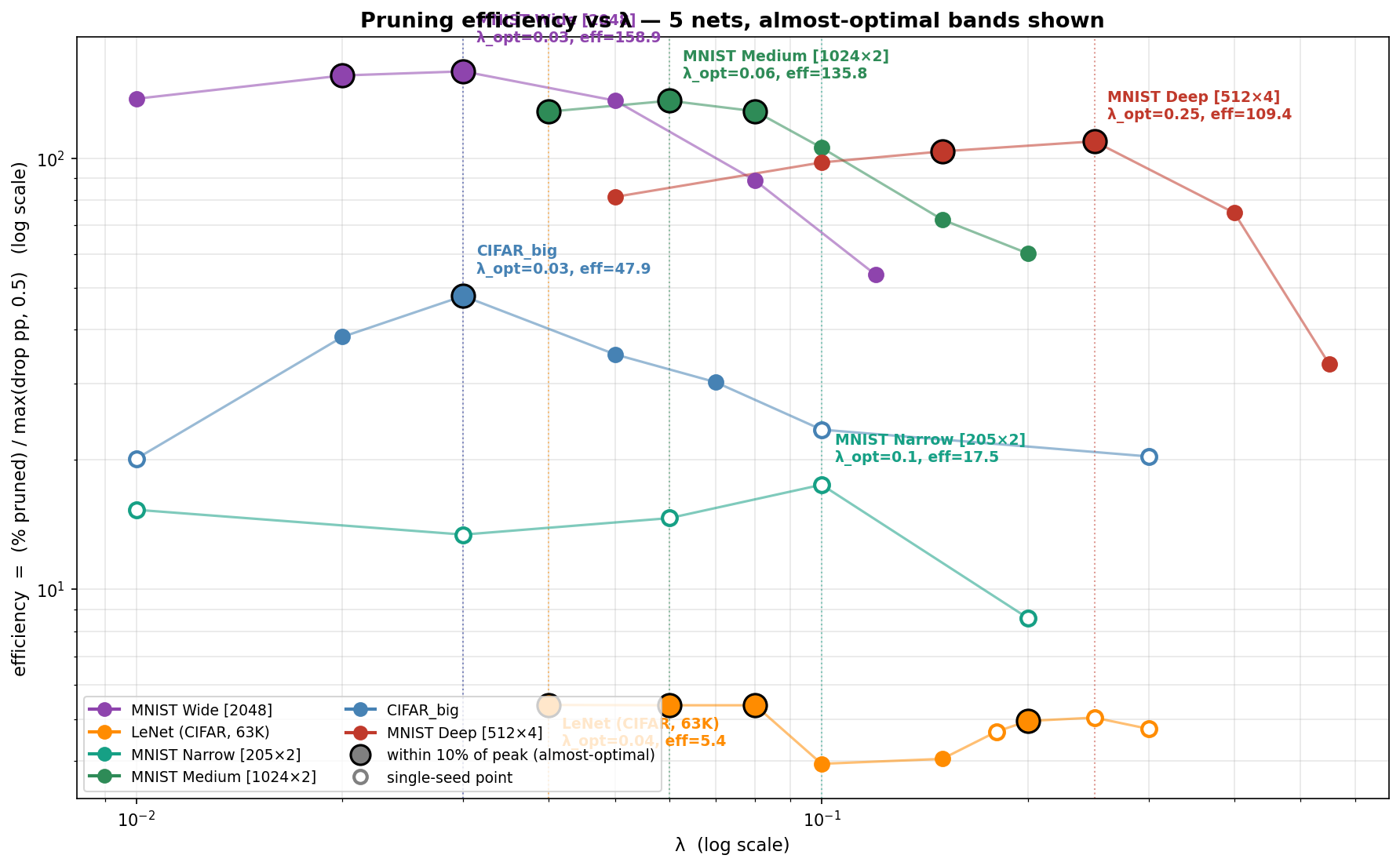
λ\lambda is the one knob, and its optimum is well-behaved. Across three base networks spanning 165×165\times in size and two datasets, the efficiency-optimal λ\lambda stays in a narrow [0.03,0.06][0.03, 0.06] band — it is not monotonic in model size.

Pruning efficiency vs lambda across five networks spanning MNIST and CIFAR

Pruning efficiency vs λ\lambda for LeNet (63K63\text{K}), MNIST MLP (1.86M1.86\text{M}), and a large CIFAR net (10.4M10.4\text{M}). λopt\lambda_{\text{opt}} stays in [0.03,0.06][0.03, 0.06] throughout; a candidate regularity λoptNlayers0.10\lambda_{\text{opt}} \cdot N_{\text{layers}} \approx 0.10 fits all three points and is cheap to falsify.

Beyond MNIST — and the Road to LLMs

Validation on CIFAR-10

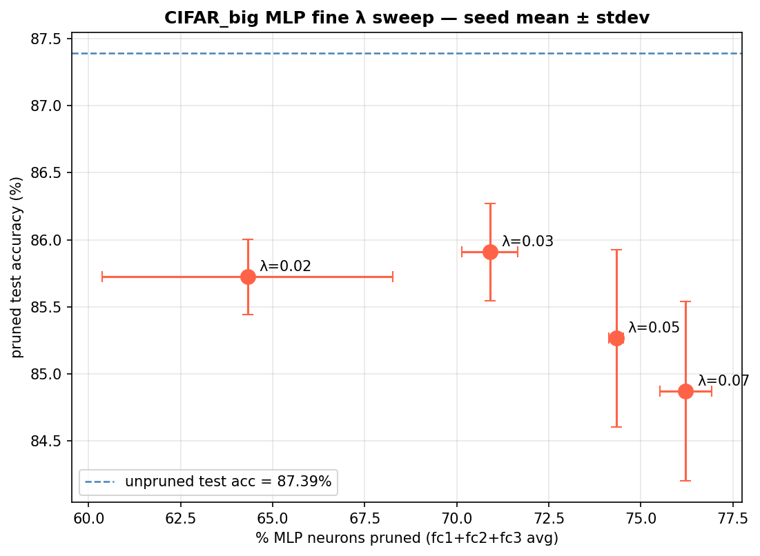
The structural findings hold beyond MNIST. On a convolutional network's MLP head on CIFAR-10, the pruner removes ~71% of head neurons at ~1.5pp cost at the Pareto knee. The width-prunability pattern reappears within a single network — the widest layer prunes hardest, while the last hidden layer before the output hits a load-bearing floor it will not cross.

CIFAR MLP-head pruning across lambda values

CIFAR MLP-head pruning across λ\lambda. The per-layer allocation mirrors the width/depth law: wide layers are compressed aggressively, the narrow pre-output layer is preserved.

Limitations

LEP characterizes redundancy in fully-connected structure — MLPs and MLP heads. Convolutional and attention layers are reached only indirectly so far. The learned mask is network-specific and does not transfer, so the method saves inference compute but not the cost of training a pruner per model. The λ\lambda-scaling regularity is supported by three data points — suggestive, not established. All accuracy numbers are at modest scale.

Research directions

We see five open lines of work:

  1. Prune during training. The single regime where the RL framing is not degenerate, because masking decisions feed back into co-adapting weights. This converts our negative RL result into a characterized boundary.

  2. A transferable redundancy detector. Meta-train LEP over a distribution of networks using permutation-invariant features. Success would turn the per-model pruner into a single reusable "redundancy reader."

  3. Prunability as an effective-dimension probe. Treat the mask as an instrument — sweep data, width, depth, and training time and read prunability off as a proxy for effective dimension, tying it quantitatively to double descent and lottery tickets.

  4. Train-to-be-prunable. A training-time regularizer that concentrates redundancy, flipping pruning from a post-hoc tool into an inductive bias.

  5. Scaling to large language models. The MLP/feed-forward blocks of transformers are exactly the fully-connected structure LEP already handles, and they hold the majority of an LLM's parameters. We intend to study whether a weight-conditioned readout finds the same kind of width-concentrated, near-deterministic redundancy in FFN blocks — and whether a per-block λ\lambda can deliver structured, inference-cheap sparsity at LLM scale. This is the direction we are most excited to pursue.

Conclusion

A trained network's redundancy is legible in its weights alone. A small weight-conditioned hypernetwork reads it out near-deterministically, beats classical heuristics at every budget, and provably outperforms RL — which on a frozen model is only static subset selection in disguise. Along the way the method surfaces a structural law: prunability tracks width, capacity tracks depth, and weights, not neurons, are conserved. Learned Efficiency Pruning is therefore as much a measurement instrument for overparameterization as it is a compression tool — and the instrument is ready to be pointed at large language models.